
• Produktbild: Time-Domain Beamforming and Blind Source Separation
  • Produktbild: Time-Domain Beamforming and Blind Source Separation
Band 3

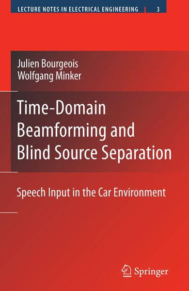
Time-Domain Beamforming and Blind Source Separation Speech Input in the Car Environment

116,99 €

inkl. gesetzl. MwSt., Versandkostenfrei


Beschreibung

Produktdetails

Einband

Taschenbuch

Erscheinungsdatum

23.11.2010

Verlag

Springer Us

Seitenzahl

225

Maße (L/B/H)

23,5/15,5/1,4 cm

Gewicht

373 g

Auflage

Softcover reprint of hardcover 1st edition 2009

Sprache

Englisch

ISBN

978-1-4419-4332-3

Beschreibung

Produktdetails

Einband

Taschenbuch

Erscheinungsdatum

23.11.2010

Verlag

Springer Us

Seitenzahl

225

Maße (L/B/H)

23,5/15,5/1,4 cm

Gewicht

373 g

Auflage

Softcover reprint of hardcover 1st edition 2009

Sprache

Englisch

ISBN

978-1-4419-4332-3

Herstelleradresse

Springer-Verlag KG
Sachsenplatz 4-6
1201 Wien
AT

Email: GPSR Kontakt

Noch keine Bewertungen vorhanden

Verfassen Sie die erste Bewertung zu diesem Artikel

Helfen Sie anderen Kundinnen und Kunden durch Ihre Meinung.

Kundinnen und Kunden meinen

Bewertungen (0)

  • Produktbild: Time-Domain Beamforming and Blind Source Separation
  • Produktbild: Time-Domain Beamforming and Blind Source Separation
  • 1 Introduction 1

    1.1 Existing approaches: a brief overview. . . . . . . . . . . . . . . . . . . . . . . . . . . . . . 1

    1.2 Scope and objective of the thesis . . . . . . . . . . . . . . . . . . . . . . . . . . . . . . . . 2

    1.3 Outline of the thesis . . . . . . . . . . . . . . . . . . . . . . . . . . . . . . . . . . . . . . . 3

    2 Non-adaptive stationary beamforming 5

    2.1 Problemand notations . . . . . . . . . . . . . . . . . . . . . . . . . . . . . . . . . . . . . . 5

    2.2 The space-frequency response for omni-directional microphones . . . . . . . . . . . . . . . 6

    2.3 Minimum VarianceDistortionless Response (MVDR) . . . . . . . . . . . . . . . . . . . . . 8

    2.4 Data-independent beamformers . . . . . . . . . . . . . . . . . . . . . . . . . . . . . . . . . 9

    2.4.1 The delay-and-sumbeamformer . . . . . . . . . . . . . . . . . . . . . . . . . . . . . 9

    2.4.2 TheMVDR null beamformer . . . . . . . . . . . . . . . . . . . . . . . . . . . . . . 10

    2.5 Statistically optimumMVDR beamformer . . . . . . . . . . . . . . . . . . . . . . . . . . . 11

    2.6 FromMVDR to Generalized Sidelobe Canceller (GSC) . . . . . . . . . . . . . . . . . . . . 12

    2.7 The target signal cancellation problem . . . . . . . . . . . . . . . . . . . . . . . . . . . . . 14

    2.7.1 The power-inversion effect . . . . . . . . . . . . . . . . . . . . . . . . . . . . . . . . 14

    2.7.2 Robust versions of the GSC . . . . . . . . . . . . . . . . . . . . . . . . . . . . . . . 15

    2.8 Use of directionalmicrophones . . . . . . . . . . . . . . . . . . . . . . . . . . . . . . . . . 15

    2.8.1 Directionalmicrophones with the same orientation . . . . . . . . . . . . . . . . . . 16

    2.8.2 Directionalmicrophones oriented to the sources . . . . . . . . . . . . . . . . . . . . 16

    2.9 Experiments under stationary acoustic conditions . . . . . . . . . . . . . . . . . . . . . . . 182.9.1 Experiments with the mirror array . . . . . . . . . . . . . . . . . . . . . . . . . . . 18

    2.9.2 Experiments with the cocooning array . . . . . . . . . . . . . . . . . . . . . . . . . 22

    2.10 Summary and conclusion . . . . . . . . . . . . . . . . . . . . . . . . . . . . . . . . . . . . 24

    3 Implicit adaptation control for beamforming 27

    3.1 Adaptive interference canceller . . . . . . . . . . . . . . . . . . . . . . . . . . . . . . . . . 27

    3.2 Implicit adaptation control with a pseudo-optimal step-size . . . . . . . . . . . . . . . . . 29

    3.3 ILMS transient behavior and stability . . . . . . . . . . . . . . . . . . . . . . . . . . . . . 31

    3.3.1 Transient convergence and divergence . . . . . . . . . . . . . . . . . . . . . . . . . 31

    3.3.2 About the stability . . . . . . . . . . . . . . . . . . . . . . . . . . . . . . . . . . . . 34

    3.4 Robustness improvement . . . . . . . . . . . . . . . . . . . . . . . . . . . . . . . . . . . . . 34

    3.5 Experiments . . . . . . . . . . . . . . . . . . . . . . . . . . . . . . . . . . . . . . . . . . . . 35

    3.5.1 Experiments with the mirror array . . . . . . . . . . . . . . . . . . . . . . . . . . . 36

    3.5.2 Experiment with the cocooning array . . . . . . . . . . . . . . . . . . . . . . . . . 38

    3.6 Summary and conclusion . . . . . . . . . . . . . . . . . . . . . . . . . . . . . . . . . . . . 40

    4 Second-Order Blind Source Separation 43

    4.1 Problemand notations . . . . . . . . . . . . . . . . . . . . . . . . . . . . . . . . . . . . . . 44

    4.1.1 Froma scalar to a convolutivemixture model . . . . . . . . . . . . . . . . . . . . . 44

    4.1.2 Separation constraints and degrees of freedom. . . . . . . . . . . . . . . . . . . . . 46

    4.2 Nonstationarity and source separation . . . . . . . . . . . . . . . . . . . . . . . . . . . . . 47

    4.2.1 The insufficiency of decorrelation . . . . . . . . . . . . . . . . . . . . . . . . . . . . 47

    i

    4.2.2 Nonstationarity-based separation cost function. . . . . . . . . . . . . . . . . . . . . 47

    4.3 Gradient-basedminimization . . . . . . . . . . . . . . . . . . . . . . . . . . . . . . . . . . 49

    4.3.1 Standard gradient . . . . . . . . . . . . . . . . . . . . . . . . . . . . . . . . . . . . 49

    4.3.2 Natural gradient . . . . . . . . . . . . . . . . . . . . . . . . . . . . . . . . . . . . . 50

    4.4 Natural gradient algorithmfor non-square systems . . . . . . . . . . . . . . . . . . . . . . 50

    4.5 Summary and conclusion . . . . . . . . . . . . . . . . . . . . . . . . . . . . . . . . . . . . 52

    5 Implementation Issues in Blind Source Separation 53

    5.1 Convolutive Natural Gradient . . . . . . . . . . . . . . . . . . . . . . . . . . . . . . . . . . 53

    5.1.1 Gradient in the Sylvestermanifold . . . . . . . . . . . . . . . . . . . . . . . . . . . 53

    5.1.2 From matrices to z-transforms . . . . . . . . . . . . . . . . . . . . . . . . . . . . . 55

    5.1.3 Self-closed and non-self-closed natural gradients . . . . . . . . . . . . . . . . . . . . 56

    5.1.4 From z-transforms back to the time domain . . . . . . . . . . . . . . . . . . . . . . 57

    5.1.5 Application to second-order BSS. . . . . . . . . . . . . . . . . . . . . . . . . . . . . 59

    5.1.6 Discussion: Which natural gradient is best? . . . . . . . . . . . . . . . . . . . . . . 60

    5.2 Online adaptation . . . . . . . . . . . . . . . . . . . . . . . . . . . . . . . . . . . . . . . . 62

    5.2.1 Blockwise batch BSS algorithm . . . . . . . . . . . . . . . . . . . . . . . . . . . . . 62

    5.2.2 Sample-wise BSS algorithm . . . . . . . . . . . . . . . . . . . . . . . . . . . . . . . 63

    5.3 Experimental results . . . . . . . . . . . . . . . . . . . . . . . . . . . . . . . . . . . . . . . 63

    5.3.1 Experiments with the mirror array . . . . . . . . . . . . . . . . . . . . . . . . . . . 64

    5.3.2 Experiments with the cocooning array . . . . . . . . . . . . . . . . . . . . . . . . . 66

    5.3.3 Comparison with other BSS algorithms in the frequency domain . . . . . . . . . . 66

    5.4 Conclusion . . . . . . . . . . . . . . . . . . . . . . . . . . . . . . . . . . . . . . . . . . . . 69

    6 Blind Source Separation: Convergence and Stability 71

    6.1 Global convergence . . . . . . . . . . . . . . . . . . . . . . . . . . . . . . . . . . . . . . . . 71

    6.1.1 Difficulty of a global convergence analysis . . . . . . . . . . . . . . . . . . . . . . . 72

    6.1.2 Convergence analysis for a simplified algorithm . . . . . . . . . . . . . . . . . . . . 73

    6.2 Local stability . . . . . . . . . . . . . . . . . . . . . . . . . . . . . . . . . . . . . . . . . . . 74

    6.3 Conclusion . . . . . . . . . . . . . . . . . . . . . . . . . . . . . . . . . . . . . . . . . . . . 76

    7 Comparison of Beamforming and Blind Source Separation 77

    7.1 System identification vs. interference cancellation . . . . . . . . . . . . . . . . . . . . . . . 77

    7.2 Properties of the cost function . . . . . . . . . . . . . . . . . . . . . . . . . . . . . . . . . 80

    7.2.1 Convergence of the gradient descent . . . . . . . . . . . . . . . . . . . . . . . . . . 80

    7.2.2 Statistical efficiency . . . . . . . . . . . . . . . . . . . . . . . . . . . . . . . . . . . 80

    7.3 Complexity . . . . . . . . . . . . . . . . . . . . . . . . . . . . . . . . . . . . . . . . . . . . 83

    7.3.1 NLMS complexity . . . . . . . . . . . . . . . . . . . . . . . . . . . . . . . . . . . . 83

    7.3.2 BSS complexity . . . . . . . . . . . . . . . . . . . . . . . . . . . . . . . . . . . . . . 84

    7.3.3 NLMS vs. BSS complexity . . . . . . . . . . . . . . . . . . . . . . . . . . . . . . . 85

    7.3.4 Online BSS algorithm in the special case N =2 . . . . . . . . . . . . . . . . . . . . 86

    7.4 Experimental comparison . . . . . . . . . . . . . . . . . . . . . . . . . . . . . . . . . . . . 87

    7.5 Summary and conclusion . . . . . . . . . . . . . . . . . . . . . . . . . . . . . . . . . . . . 89

    8 Combining Blind Source Separation and Beamforming 91

    8.1 Existing combinations . . . . . . . . . . . . . . . . . . . . . . . . . . . . . . . . . . . . . . 91

    8.2 BSS and geometric prior information . . . . . . . . . . . . . . . . . . . . . . . . . . . . . . 92

    8.2.1 Causality information . . . . . . . . . . . . . . . . . . . . . . . . . . . . . . . . . . 92

    8.2.2 Prior information on the source direction of arrival . . . . . . . . . . . . . . . . . . 93

    8.2.3 Geometric information at the initialization . . . . . . . . . . . . . . . . . . . . . . 95

    8.2.4 Geometric information as a soft constraint . . . . . . . . . . . . . . . . . . . . . . . 96

    8.2.5 Geometric information as a preprocessing . . . . . . . . . . . . . . . . . . . . . . . 99

    8.3 Combining BSS and the power criterion . . . . . . . . . . . . . . . . . . . . . . . . . . . . 101

    8.4 Combining BSS with geometric prior information and the power criterion . . . . . . . . . 102

    ii

    8.5 Experimental results on automatic speech recognition . . . . . . . . . . . . . . . . . . . . 104

    8.6 Conclusion . . . . . . . . . . . . . . . . . . . . . . . . . . . . . . . . . . . . . . . . . . . . 105

    A Experimental setups 109

    A.1 Mirror array . . . . . . . . . . . . . . . . . . . . . . . . . . . . . . . . . . . . . . . . . . . . 109

    A.2 Cocooning array . . . . . . . . . . . . . . . . . . . . . . . . . . . . . . . . . . . . . . . . . 109

    A.3 Acoustic characteristics of the car cabin. . . . . . . . . . . . . . . . . . . . . . . . . . . . . 111

    B The RGSC according to Hoshuyama et al. 113

    B.1 RGSC for the mirror array . . . . . . . . . . . . . . . . . . . . . . . . . . . . . . . . . . . 113

    B.2 RGSC for the cocooning array. . . . . . . . . . . . . . . . . . . . . . . . . . . . . . . . . . 114

    B.3 Experimental comparison: GSC vs. RGSC. . . . . . . . . . . . . . . . . . . . . . . . . . . 115

    B.3.1 Mirror array . . . . . . . . . . . . . . . . . . . . . . . . . . . . . . . . . . . . . . . 115

    B.3.2 Cocooning array. . . . . . . . . . . . . . . . . . . . . . . . . . . . . . . . . . . . . . 115

    B.4 Conclusion . . . . . . . . . . . . . . . . . . . . . . . . . . . . . . . . . . . . . . . . . . . . 115

    C Stability Analysis 119

    C.1 Mixing and separationmodels . . . . . . . . . . . . . . . . . . . . . . . . . . . . . . . . . . 119

    C.2 Linearization of the BSS updates . . . . . . . . . . . . . . . . . . . . . . . . . . . . . . . . 120

    C.3 Local stability conditions . . . . . . . . . . . . . . . . . . . . . . . . . . . . . . . . . . . . 122

    Bibliography 125

    iii