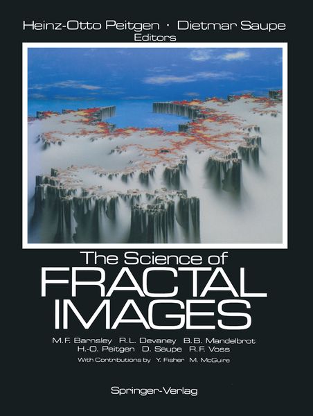

• Produktbild: The Science of Fractal Images
  • Produktbild: The Science of Fractal Images

The Science of Fractal Images

105,99 €

inkl. gesetzl. MwSt., Versandkostenfrei


Beschreibung

Produktdetails

Einband

Taschenbuch

Erscheinungsdatum

08.10.2011

Herausgeber

Heinz-Otto Peitgen + weitere

Verlag

Springer Us

Seitenzahl

312

Maße (L/B/H)

28/21/1,9 cm

Gewicht

815 g

Auflage

Softcover reprint of the original 1st ed. 1988

Sprache

Englisch

ISBN

978-1-4612-8349-2

Beschreibung

Portrait

Benoit B. Mandelbrot, geb. 1924 in Warschau, arbeitete als Mathematiker lange Zeit bei IBM, ist Honorarprofessor an der Yale University und Erfinder der fraktalen Geometrie. Mandelbrot lebt in Scarsdale, New York.

Produktdetails

Einband

Taschenbuch

Erscheinungsdatum

08.10.2011

Herausgeber

Verlag

Springer Us

Seitenzahl

312

Maße (L/B/H)

28/21/1,9 cm

Gewicht

815 g

Auflage

Softcover reprint of the original 1st ed. 1988

Sprache

Englisch

ISBN

978-1-4612-8349-2

Herstelleradresse

Springer-Verlag KG
Sachsenplatz 4-6
1201 Wien
AT

Email: GPSR Kontakt

Noch keine Bewertungen vorhanden

Verfassen Sie die erste Bewertung zu diesem Artikel

Helfen Sie anderen Kundinnen und Kunden durch Ihre Meinung.

Kundinnen und Kunden meinen

Bewertungen (0)

  • Produktbild: The Science of Fractal Images
  • Produktbild: The Science of Fractal Images
  • 1 Fractals in nature: From characterization to simulation.- 1.1 Visual introduction to fractals: Coastlines, mountains and clouds.- 1.1.1 Mathematical monsters: The fractal heritage.- 1.1.2 Fractals and self-similarity.- 1.1.3 An early monster: The von Koch snowflake curve.- 1.1.4 Self-similarity and dimension.- 1.1.5 Statistical self-similarity.- 1.1.6 Mandelbrot landscapes.- 1.1.7 Fractally distributed craters.- 1.1.8 Fractal planet: Brownian motion on a sphere.- 1.1.9 Fractal flakes and clouds.- 1.2 Fractals in nature: A brief survey from aggregation to music.- 1.2.1 Fractals at large scales.- 1.2.2 Fractals at small scales: Condensing matter.- 1.2.3 Scaling randomness in time: 1/f?-noises.- 1.2.4 Fractal music.- 1.3 Mathematical models: Fractional Brownian motion.- 1.3.1 Self-affinity.- 1.3.2 Zerosets.- 1.3.3 Self-affinity in higher dimensions : Mandelbrot landscapes and clouds.- 1.3.4 Spectral densities for fBm and the spectral exponent ?.- 1.4 Algorithms: Approximating fBm on a finite grid.- 1.4.1 Brownian motion as independent cuts.- 1.4.2 Fast Fourier Transform filtering.- 1.4.3 Random midpoint displacement.- 1.4.4 Successive random additions.- 1.4.5 Weierstrass-Mandelbrot random fractal function.- 1.5 Laputa: A concluding tale.- 1.6 Mathematical details and formalism.- 1.6.1 Fractional Brownian motion.- 1.6.2 Exact and statistical self-similarity.- 1.6.3 Measuring the fractal dimension D.- 1.6.4 Self-affinity.- 1.6.5 The relation of D to H for self-affine fractional Brownian motion.- 1.6.6 Trails of fBm.- 1.6.7 Self-affinity in E dimensions.- 1.6.8 Spectral densities for fBm and the spectral exponent ?.- 1.6.9 Measuring fractal dimensions: Mandelbrot measures.- 1.6.10 Lacunarity.- 1.6.11 Random cuts with H ? 1/2: Campbell’s theorem.- 1.6.12 FFT filtering in 2 and 3 dimensions.- 2 Algorithms for random fractals.- 2.1 Introduction.- 2.2 First case study: One-dimensional Brownian motion.- 2.2.1 Definitions.- 2.2.2 Integrating white noise.- 2.2.3 Generating Gaussian random numbers.- 2.2.4 Random midpoint displacement method.- 2.2.5 Independent jumps.- 2.3 Fractional Brownian motion : Approximation by spatial methods.- 2.3.1 Definitions.- 2.3.2 Midpoint displacement methods.- 2.3.3 Displacing interpolated points.- 2.4 Fractional Brownian motion : Approximation by spectral synthesis.- 2.4.1 The spectral representation of random functions.- 2.4.2 The spectral exponent ? in fractional Brownian motion.- 2.4.3 The Fourier filtering method.- 2.5 Extensions to higher dimensions.- 2.5.1 Definitions.- 2.5.2 Displacement methods.- 2.5.3 The Fourier filtering method.- 2.6 Generalized stochastic subdivision and spectral synthesis of ocean waves.- 2.7 Computer graphics for smooth and fractal surfaces.- 2.7.1 Top view with color mapped elevations.- 2.7.2 Extended floating horizon method.- Color plates and captions.- 2.7.3 The data and the projection.- 2.7.4 A simple illumination model.- 2.7.5 The rendering.- 2.7.6 Data manipulation.- 2.7.7 Color, anti-aliasing and shadows.- 2.7.8 Data storage considerations.- 2.8 Random variables and random functions.- 3 Fractal patterns arising in chaotic dynamical systems.- 3.1 Introduction.- 3.1.1 Dynamical systems.- 3.1.2 An example from ecology.- 3.1.3 Iteration.- 3.1.4 Orbits.- 3.2 Chaotic dynamical systems.- 3.2.1 Instability: The chaotic set.- 3.2.2 A chaotic set in the plane.- 3.2.3 A chaotic gingerbreadman.- 3.3 Complex dynamical systems.- 3.3.1 Complex maps.- 3.3.2 The Julia set.- 3.3.3 Julia sets as basin boundaries.- 3.3.4 Other Julia sets.- 3.3.5 Exploding Julia sets.- 3.3.6 Intermittency.- 4 Fantastic deterministic fractals.- 4.1 Introduction.- 4.2 The quadratic family.- 4.2.1 The Mandelbrot set.- 4.2.2 Hunting for Kc in the plane — the role of critical points.- 4.2.3 Level sets.- 4.2.4 Equipotential curves.- 4.2.5 Distance estimators.- 4.2.6 External angles and binary decompositions.- 4.2.7 Mandelbrot set as one-page-dictionary of Julia sets.- 4.3 Generalizations and extensions.- 4.3.1 Newton’s Method.- 4.3.2 Sullivan classification.- 4.3.3 The quadratic family revisited.- 4.3.4 Polynomials.- 4.3.5 A special map of degree four.- 4.3.6 Newton’s method for real equations.- 4.3.7 Special effects.- 5 Fractal modelling of real world images.- 5.1 Introduction.- 5.2 Background references and introductory comments.- 5.3 Intuitive introduction to IFS: Chaos and measures.- 5.3.1 The Chaos Game : ‘Heads’, ‘Tails’ and ‘Side’.- 5.3.2 How two ivy leaves lying on a sheet of paper can specify an affine transformation.- 5.4 The computation of images from IFS codes.- 5.4.1 What an IFS code is.- 5.4.2 The underlying model associated with an IFS code.- 5.4.3 How images are defined from the underlying model.- 5.4.4 The algorithm for computing rendered images.- 5.5 Determination of IFS codes: The Collage Theorem.- 5.6 Demonstrations.- 5.6.1 Clouds.- 5.6.2 Landscape with chimneys and smoke.- 5.6.3 Vegetation.- A Fractal landscapes without creases and with rivers.- A.1 Non-Gaussian and non-random variants of midpoint displacement.- A.1.1 Midpoint displacement constructions for the paraboloids.- A.1.2 Midpoint displacement and systematic fractals: The Takagi fractal curve, its kin, and the related surfaces.- A.1.3 Random midpoint displacements with a sharply non-Gaussian displacements’ distribution.- A.2 Random landscapes without creases.- A.2.1 A classification of subdivision schemes: One may displace the midpoints of either frame wires or of tiles.- A.2.2 Context independence and the “creased” texture.- A.2.3 A new algorithm using triangular tile midpoint displacement.- A.2.4 A new algorithm using hexagonal tile midpoint displacement.- A.3 Random landscape built on prescribed river networks.- A.3.1 Building on a non-random map made of straight rivers and watersheds, with square drainage basins.- A.3.2 Building on the non-random map shown on the top of Plate 73 of “The Fractal Geometry of Nature”.- B An eye for fractals.- Dietmar Saupe.- C A unified approach to fractal curves and plants.- C.1 String rewriting systems.- C.2 The von Koch snowflake curve revisited.- C.3 Formal definitions and implementation.- D Exploring the Mandelbrot set.- B An eye for fractals.- Yuval Fisher.- D.1 Bounding the distance to M.- D.2 Finding disks in the interior of M.- D.3 Connected Julia sets.